For an assignment in a machine learning class, we were given a file with 95,000 movie ratings in the form of - user_id, movie_id and rating. From this we can build what is called an incomplete ratings matrix and the assignment was to fill in the matrix using probabilistic matrix factorization which is a form of collaborative filtering. There are 1,682 different movies and 943 different users in the data. Since we have 95,000 ratings, there are 1.5 million incomplete (missing) ratings or 94%. Here is an example of a ratings matrix. In practice, there are more blanks.

To perform matrix factorization, we decide on a number of features (e.g., 10), and factorize the ratings matrix into two matrices, one for the movies and one for the users, each with 10 dimensions (the number of features we settled on). Each row of the movie matrix corresponds to one movie and we learn 10 numbers for each movie, a movie vector. Similarly, each row of the user matrix corresponds to one user and we learn 10 numbers for each user, a user vector. It is an iterative process where we first update each user vector based on each movie they have rated, and the rating they gave it and then update each movie vector based on the information we have about each user who rated this movie (which is contained in the user vector) and the rating that user gave. We repeat this process until the changes in the movie and user vectors drop below some threshold. The code is at the bottom of this post and on my GitHub page. The idea is that once we have learned the two matrices, we can predict a missing value in the ratings matrix using the respective movie and user vectors. For example, if we want to predict how Erica would rate Pulp Fiction, we would multiply the row of the user matrix corresponding to Erica by the row of the movie matrix corresponding to Pulp Fiction.
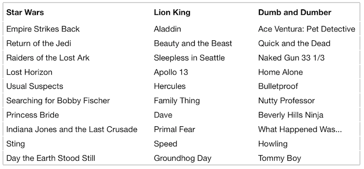
A nice way to test whether the 10-numbers (features) that we have learned have any meaning, is to see if similar movies have similar values for the 10 features. To do so, we select a movie, and then calculate its distance to every other movie (distance is essentially the sum of the respective differences in the 10 numbers). Here are the 10 movies closest to ‘Star Wars’, ‘Lion King’ and ‘Dumb and Dumber’.

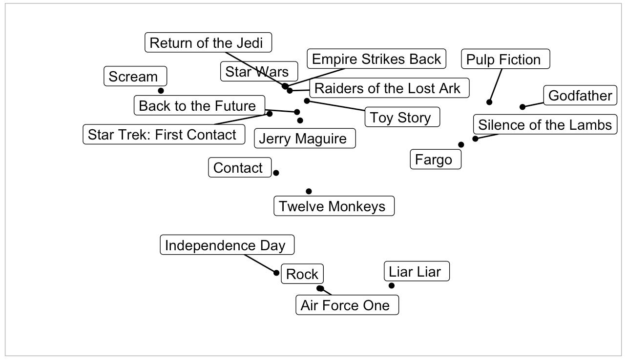
If we were able to visualize a 10-dimensional space, these would be the ten movies that are closest to the given movie in that space. To view it in 2D, we can use a feature of scikit-learn called t-SNE to perform dimensionality reduction and reduce each movie to 2-dimensions. As this resulted in many points that were extremely close to each other, I used the ggrepel library in R to separate the data points.

The three Star Wars movies are right next to each other, same with The Rock, Independence Day and Air Force One, but what is Liar Liar doing so close by? It’s nice to be able to compare the movies in a scatterplot but we lost information.
Back to 10-dimensions, I was curious if I could understand what the 10 factors that the model learns actually capture. To investigate this, I looked at what movies had the highest and lowest values for each of the ten factors. When I did this the first time, I didn’t recognize most of the movies, so I only considered the 250 movies with the highest number of ratings. I had trouble deciphering many of the factors but found these two to be clear.

The factor on the left captures dark vs. romantic with crime dramas high in the factor and romantic dramas low in the factor. The right factor appears to be musical/comedy vs. action. Pretty amazing that this information can be extracted from 95,000 movie ratings. Netflix has a lot more than that.
The ratings data was adapted from the GroupLens Research Project at the University of Minnesota by John Paisley, the professor of my Machine Learning course. I used Python to iteratively build the movie and user matrices and ggplot to plot the movie locations.